Analyzing Asynchronous Systems with Timing Diagrams

In modern digital design, understanding the flow of signals across time is critical for ensuring system reliability. Asynchronous systems, where operations are not governed by a single global clock, present unique challenges compared to synchronous counterparts. The primary tool used to visualize and debug these complex interactions is the timing diagram. This guide provides a deep dive into how to construct, read, and analyze timing diagrams within asynchronous environments.

The Nature of Asynchronous Design 🌐

Asynchronous systems operate without a centralized clock signal driving every state change. Instead, events are triggered by the completion of previous operations or the arrival of data. This approach offers benefits such as reduced power consumption and higher potential performance in specific contexts. However, it introduces complexity regarding signal synchronization and timing verification.

When engineers analyze these systems, they must account for variable delays, propagation times, and the lack of a universal reference point. Timing diagrams serve as the visual language to map these events. They allow teams to see the exact relationship between signal transitions over time.

Anatomy of a Timing Diagram 📐

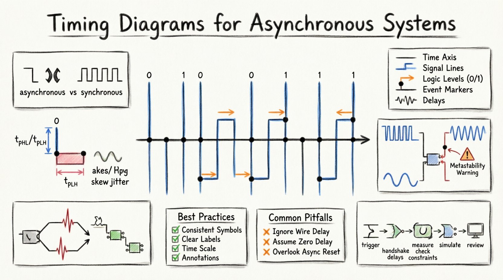
A timing diagram is a graphical representation of signal behavior. It plots time along the horizontal axis and signal states along the vertical axis. To analyze an asynchronous system effectively, one must understand the fundamental components that make up these diagrams.

• Time Axis: Represents the progression of time. In asynchronous analysis, this is often relative to a specific event trigger rather than a clock cycle.
• Signal Lines: Horizontal lines representing individual wires or nets. Each line tracks the logic level (High, Low, or Unknown) of a specific signal.
• Logic Levels: Typically denoted as 0 (Low/Ground) and 1 (High/VCC). Transitions between these states are the core of the analysis.
• Event Markers: Vertical lines or annotations indicating specific occurrences, such as a handshake signal changing state.
• Delays: Visual gaps between an input change and the corresponding output change, representing propagation delay.

Unlike synchronous diagrams which rely on grid lines representing clock edges, asynchronous diagrams rely on event boundaries. This requires a more careful interpretation of the spacing between transitions.

Critical Timing Parameters ⚙️

To analyze the integrity of an asynchronous system, specific timing parameters must be measured and compared against design specifications. These parameters define the window in which a signal must be stable to be correctly interpreted by a receiver.

Propagation Delay

Propagation delay is the time it takes for a signal to travel from the input of a component to its output. In asynchronous logic, this delay is a primary source of uncertainty. Variations in manufacturing, temperature, and voltage can alter this delay.

• tpHL: Time for a signal to transition from High to Low.
• tpLH: Time for a signal to transition from Low to High.
• tpd: General propagation delay, often calculated as the average of tpHL and tpLH.

When analyzing a timing diagram, look for the horizontal distance between the input edge and the resulting output edge. This distance is the propagation delay.

Setup and Hold Time

Even in asynchronous systems, flip-flops and latches often require specific windows of stability. Setup time is the duration before a triggering event that the data must be stable. Hold time is the duration after the triggering event that the data must remain stable.

If these windows are violated, the system may enter a state of metastability, where the output is neither High nor Low, but an undefined voltage level. Timing diagrams help visualize these violations by showing if data changes too close to a control edge.

Skew and Jitter

• S skew: The difference in arrival time of the same signal at two different points in the circuit.
• Jitter: Short-term variations in the signal timing. In asynchronous systems, jitter can be caused by power noise or crosstalk.

Handling Clock Domain Crossings 🔄

One of the most common sources of errors in mixed-mode systems involves crossing between different clock domains. Even if a system is primarily asynchronous, it often contains synchronous sub-blocks operating at different frequencies. Timing diagrams are essential for verifying these crossings.

When a signal moves from one clock domain to another, the receiver may sample the signal at a time when the signal is changing. This leads to metastability. The standard approach to mitigate this is using a synchronizer, typically a chain of flip-flops.

Parameter	Description	Impact on Timing Diagram
Metastability Resolution Time	Time required for the synchronizer to resolve to a valid logic level	Shows an extended period of undefined state before the signal stabilizes
Cross Domain Latency	Additional delay introduced by the synchronizer	Increases the time gap between the source event and the destination event
Handshake Latency	Time taken for acknowledgment signals in async protocols	Creates a back-and-forth pattern in the signal timeline

Analysts must ensure that the timing diagram accounts for the resolution time. If a downstream block attempts to read the signal before the synchronizer resolves, data corruption occurs.

Identifying and Resolving Race Conditions ⚠️

A race condition occurs when the system behavior depends on the relative timing of events that should not influence each other. In asynchronous logic, this is a frequent concern. Timing diagrams are the primary method for detecting these conditions.

Static Hazards

A static hazard occurs when a signal should remain at a constant level but momentarily flips due to path delays. For example, if a signal is logically supposed to stay High, but a change in input causes a brief dip to Low, this is a static-1 hazard.

• Visual Indicator: A narrow spike or pulse on a signal line that should be flat.
• Root Cause: Unequal propagation delays through different logic gates.

Dynamic Hazards

Dynamic hazards involve multiple transitions when only one is expected. This often happens in complex logic paths where signals travel through different numbers of gates.

Analysis Steps for Race Conditions

1. Trace the Paths: Identify all paths a signal takes from source to destination.
2. Measure Delays: Calculate the delay for each path using the timing diagram.
3. Compare Edges: Check if the arrival times of competing signals overlap in a way that creates ambiguity.
4. Verify Stability: Ensure that control signals remain stable during the critical window of data arrival.

If a race condition is found, the design may need to be restructured. Common solutions include adding buffers to equalize delays, inserting handshake protocols, or using asynchronous FIFO structures.

Signal Integrity and Noise Considerations 🔌

Timing diagrams do not exist in a vacuum. The physical layer introduces noise that affects signal quality. When analyzing asynchronous systems, engineers must distinguish between logical timing errors and physical signal degradation.

Signal Glitches

Glitches are short-lived pulses that can propagate through a circuit. In asynchronous systems, a glitch can trigger a latch or flip-flop erroneously. Timing diagrams often show these as thin spikes.

• Filtering: Ensure downstream logic has enough delay to filter out these pulses.
• Edge Rate: Steeper edges (faster rise/fall times) are more susceptible to noise coupling.

Crosstalk

Crosstalk occurs when a signal on one wire induces a voltage on an adjacent wire. This can shift the timing of a signal, causing it to arrive earlier or later than expected.

In a timing diagram, crosstalk might manifest as a shift in the edge location or an additional noise spike. To mitigate this, spacing between signals must be considered during the physical design phase.

Best Practices for Documentation 📝

Clear documentation ensures that the timing analysis can be reproduced and understood by other engineers. A well-structured timing diagram includes specific metadata and annotations.

Standardization

• Use consistent symbols for logic levels.
• Label all signals clearly with their function.
• Indicate the time scale explicitly (e.g., nanoseconds per division).

Annotations

Text annotations are crucial for explaining specific behaviors. Use arrows to point out critical transitions or potential problem areas. Label the propagation delay values directly on the diagram.

Version Control

Timing diagrams evolve as the design changes. Maintain version numbers for all diagrams to ensure that the analysis matches the current hardware state. Do not rely on memory for timing details.

Step-by-Step Analysis Process 🛠️

To effectively analyze an asynchronous system, follow a structured approach. This ensures that no critical timing parameter is overlooked.

1. Define the Trigger: Identify the event that initiates the sequence. This is usually the starting point for the time axis.
2. Map the Handshake: Trace the request and acknowledge signals. Ensure they follow the correct protocol (e.g., four-phase or two-phase handshake).
3. Measure Delays: Calculate the total latency from the trigger to the final output. Break this down into component delays.
4. Check Constraints: Verify that setup and hold times are met for all storage elements involved.
5. Simulate Variations: Analyze the diagram under worst-case conditions, such as maximum temperature or minimum voltage.
6. Review Metastability: Ensure that the probability of metastability is reduced to an acceptable level through synchronizers.

Common Pitfalls in Timing Analysis ⚡

Even experienced engineers can miss subtle issues. Being aware of common pitfalls helps avoid costly redesigns.

• Ignoring Wire Delay: Relying solely on gate delay while neglecting the resistance and capacitance of the interconnects.
• Assuming Zero Delay: Treating feedback loops as instantaneous, which is physically impossible.
• Overlooking Asynchronous Reset: Failing to account for the timing of reset signals relative to data signals.
• Confusing Edge and Level: Mixing up edge-triggered and level-triggered behaviors in the diagram interpretation.

Conclusion on Verification ✅

Timing diagrams are indispensable for the verification of asynchronous systems. They provide a concrete visual representation of abstract timing relationships. By rigorously analyzing these diagrams, engineers can identify race conditions, verify handshake protocols, and ensure signal integrity.

The complexity of asynchronous design demands precision. Every nanosecond counts. A thorough understanding of propagation delays, setup times, and hold times allows for the creation of robust systems. While the lack of a global clock adds difficulty, the insights gained from detailed timing analysis lead to more efficient and reliable designs.

Continuing to refine these analysis skills ensures that systems perform correctly under varying environmental conditions. The goal is stability and predictability, achieved through meticulous documentation and measurement.

Advanced Considerations 🔬

For high-performance applications, additional factors come into play. These include temperature gradients across the chip and voltage droop during switching events.

• Temperature Gradients: Signals traveling from the hot center of a chip to the cooler edge will experience different speeds. This variation must be reflected in the timing analysis.
• Power Grid Noise: Simultaneous switching noise can shift logic thresholds. Timing diagrams should ideally include a representation of power rail stability.
• Variable Latency: Some asynchronous protocols allow for variable latency. The timing diagram must show the range of acceptable latencies, not just a single value.

By incorporating these advanced considerations, the timing analysis becomes a comprehensive tool for system validation. It moves beyond simple verification to true performance optimization.

Remember that timing is not just about speed; it is about correctness. A fast system that fails due to timing errors is less useful than a slower system that functions reliably. The timing diagram is the map that guides you to that reliability.