Accurate project estimation is a cornerstone of successful software development. When planning a system, understanding the underlying data movements provides a concrete foundation for predicting resource requirements. The Data Flow Diagram (DFD) serves as a powerful visual tool to map these movements. By analyzing the structural complexity of a DFD, teams can derive more reliable effort estimates than relying solely on functional requirements.
This guide explores how to leverage DFD complexity metrics to refine effort estimation. We will examine the components that drive complexity, methods for quantifying these elements, and the process of translating diagrammatic analysis into project timelines.
🔍 Understanding Data Flow Diagrams in Planning
A Data Flow Diagram is a graphical representation of the flow of data through an information system. Unlike flowcharts that focus on control logic, DFDs focus on data transformation. In the context of estimation, a DFD acts as a blueprint for the work involved.
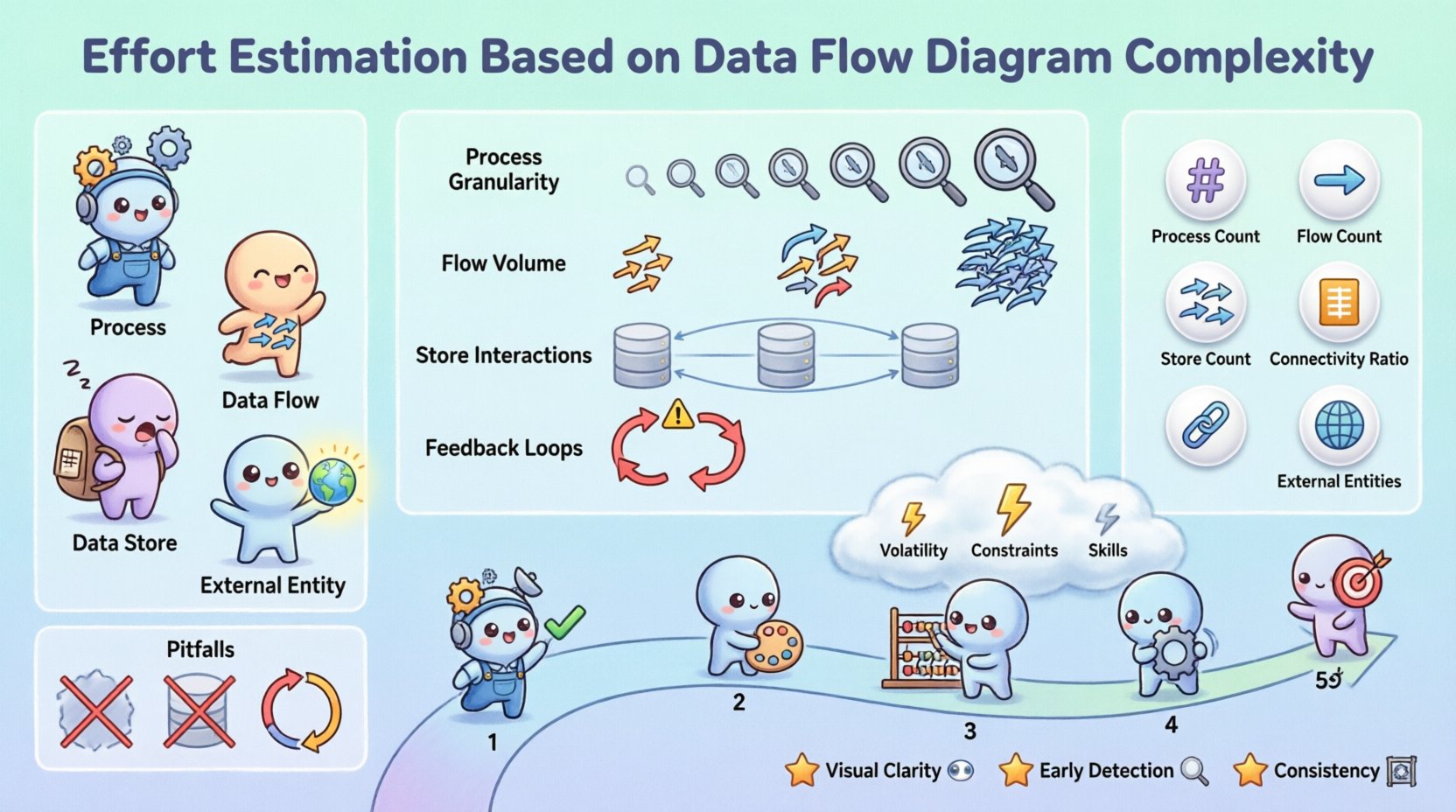
- Processes: Represent transformations of data. Each process typically maps to a specific function or module in the code.
- Data Flows: Show the movement of data between processes, stores, and entities. These represent the interfaces and integration points.
- Data Stores: Indicate where data is held at rest. These correspond to database tables or file systems.
- External Entities: Sources or destinations of data outside the system. These define integration requirements.
When estimating effort, the visual density and connectivity of these elements provide clues about the cognitive load required to implement the system. A sparse diagram with linear flows suggests lower complexity, while a dense web of interactions implies significant integration challenges.
🏗️ Identifying Complexity Drivers
Not all data flows are created equal. Some represent simple field transfers, while others involve complex business logic, validation, or security protocols. To estimate accurately, you must identify the specific drivers that increase complexity within the diagram.
1. Process Granularity
The level of detail in a process matters. A high-level process like “Process Order” might hide dozens of sub-steps. If the DFD is at a high level, the estimation must account for the decomposition of that process. Conversely, a detailed level 2 or 3 DFD reveals the actual work units.
- Coarse-grained processes: Require more analysis time to decompose.
- Fine-grained processes: Allow for more direct estimation but may miss integration overhead.
2. Data Flow Volume
The number of arrows connecting elements indicates the volume of data handling. Each arrow represents a data structure that must be validated, transformed, and stored or transmitted.
- More flows often mean more API endpoints or database queries.
- Complex flows may require error handling and retry logic.
3. Data Store Interactions
Every interaction with a data store introduces latency considerations, concurrency issues, and schema management. A process that reads and writes to multiple stores simultaneously is more complex than one interacting with a single store.
4. Feedback Loops
Loops in the diagram indicate iterative processing or state changes. These are often the most error-prone areas of development. Estimating for loops requires accounting for testing scenarios where state is maintained across multiple cycles.
📏 Quantitative Metrics for Estimation
To move from qualitative observations to quantitative estimates, specific metrics derived from the DFD can be applied. These metrics help standardize the estimation process across different projects.
| Metric | Description | Impact on Effort |
|---|---|---|
| Process Count | Total number of transformation nodes. | Direct correlation to function points. |
| Flow Count | Total number of data movement arrows. | Indicates integration and interface complexity. |
| Store Count | Total number of data repositories. | Impacts database design and migration effort. |
| Connectivity Ratio | Ratio of flows to processes. | High ratios suggest tightly coupled systems. |
| External Entity Count | Number of external systems involved. | Increases communication and dependency risk. |
By summing these values, you can create a complexity score. For example, a simple system might have 5 processes and 10 flows, while a complex system could have 50 processes and 150 flows. This score can then be multiplied by a baseline effort factor determined by historical data.
🛠️ The Estimation Process
Translating a DFD into an effort estimate requires a structured approach. Follow these steps to ensure consistency and accuracy in your planning.
Step 1: Validate Diagram Completeness
Before estimating, ensure the DFD accurately reflects the requirements. Missing flows or entities will lead to underestimation. Check that every data requirement has a corresponding flow and that every process has a defined input and output.
Step 2: Categorize Process Complexity
Not all processes require the same amount of effort. Assign a complexity weight to each process based on its logic.
- Simple: Direct data mapping or retrieval. (Weight: 1)
- Medium: Includes validation, calculation, or formatting. (Weight: 2)
- Complex: Involves multiple data stores, external APIs, or complex algorithms. (Weight: 3)
Step 3: Calculate Base Effort
Multiply the number of processes in each category by their respective weights. Sum these values to get the Base Complexity Score (BCS).
Formula: BCS = (Simple Count × 1) + (Medium Count × 2) + (Complex Count × 3)
Step 4: Adjust for Flow Complexity
High volumes of data flow increase the effort required for interface development. Apply a flow multiplier based on the total flow count relative to the process count.
- Low Ratio (≤ 2 flows per process): Multiplier 1.0
- Medium Ratio (3-5 flows per process): Multiplier 1.2
- High Ratio (> 5 flows per process): Multiplier 1.5
Step 5: Factor in External Dependencies
External entities introduce risk. Each external system requires integration testing, security configuration, and potential vendor coordination. Add a fixed time buffer for each external entity.
⚠️ Adjusting for Risk and Uncertainty
Even with a detailed DFD, uncertainty remains. Factors such as changing requirements or technical debt can alter the effort required. Adjust your estimates to account for these risks.
1. Requirement Volatility
If the business requirements are likely to change during development, the DFD may need significant revision. In such cases, add a contingency buffer of 15-20% to the total effort.
2. Technical Constraints
Legacy systems or specific infrastructure requirements can complicate data flows. If the DFD shows data moving to a legacy mainframe, the effort to handle that connection may be higher than standard API calls.
3. Skill Level of Team
Estimation assumes a baseline competence. If the team is new to the domain or the technology stack, the complexity of the DFD processes may translate to more learning time. Adjust the time per process unit accordingly.
🚫 Common Pitfalls in DFD Analysis
Avoiding common mistakes is crucial for maintaining estimation integrity. Several traps can lead to significant miscalculations.
- Ignoring Data Validation: A DFD shows data moving, but not the rules applied to it. Validation logic often accounts for 20-30% of process effort.
- Overlooking Error Handling: Happy paths are easy to map. Error paths, retries, and logging add hidden complexity to every flow.
- Assuming Linear Growth: Complexity often grows non-linearly. Adding one more data store can increase connection complexity exponentially due to the need for transaction consistency.
- Neglecting Security: Encryption, authentication, and authorization layers are often implicit in DFDs. Explicitly account for these in the estimation.
- Focusing Only on Processes: Data stores and flows are often more time-consuming to set up and test than the processes themselves.
📅 Integrating Estimates into Project Schedules
Once the effort is calculated, it must be mapped to a schedule. This involves resource allocation and milestone definition.
- Phased Delivery: Group processes by data flow dependencies. Deliver high-priority flows first to reduce risk.
- Parallel Workstreams: If processes are independent, they can be developed in parallel. Use the DFD to identify independent clusters.
- Integration Testing: Schedule dedicated time for testing data flow integrity. This is often where complex DFDs fail.
By aligning the schedule with the structural dependencies shown in the diagram, you create a realistic timeline that respects the natural flow of the system.
🔄 Maintaining Accuracy Over Time
Estimates are not static. As the project progresses and the DFD evolves, the estimates should be recalibrated.
- Baseline Updates: When the DFD is finalized, update the initial estimates with the actual complexity scores.
- Retrospective Analysis: After a phase, compare the estimated complexity score against the actual effort spent. This refines the weighting factors for future projects.
- Change Management: Any change to the DFD should trigger a re-estimation. Do not assume that adding a small flow has negligible impact.
🛡️ Final Considerations for DFD-Based Planning
Using Data Flow Diagrams for effort estimation provides a structured, objective method to gauge project size. It moves the conversation away from guesswork and towards analysis of the system’s actual data architecture.
While no model is perfect, the DFD complexity approach offers significant advantages:
- Visual Clarity: Stakeholders can see the data movement, making the effort justification transparent.
- Early Detection: Complex flows can be identified before coding begins, allowing for architectural adjustments.
- Consistency: Applying the same metrics across different projects allows for better portfolio management.
Remember that the goal is not perfection, but informed planning. Regularly review your complexity factors and update your baselines. As your team gains experience with specific types of flows and processes, your ability to predict effort will improve naturally.
By treating the DFD as a primary estimator, you align your planning with the fundamental nature of the system you are building. This leads to more realistic budgets, schedules, and ultimately, more successful delivery of software solutions.