In the complex architecture of modern distributed systems, time is not merely a metric to be measured; it is a fundamental constraint that dictates system behavior. Software reliability is not solely about preventing crashes or handling exceptions; it is about ensuring that components interact correctly within specific temporal boundaries. When multiple threads, services, or hardware devices attempt to access shared resources, the sequence and duration of these interactions become critical. This is where timing diagrams become indispensable.
Timing diagrams provide a visual representation of how signals or messages change state over time. They allow engineers to model the temporal relationships between events before a single line of code is executed. By visualizing the flow of time, teams can identify potential bottlenecks, race conditions, and synchronization errors that are often invisible in static flowcharts or sequence diagrams. This guide explores the mechanics of using timing diagrams to enhance software reliability, offering a deep dive into concurrency, latency analysis, and system validation.
🔍 Defining Timing Diagrams in Engineering
A timing diagram is a type of behavioral diagram in system modeling that describes the behavior of objects over time. Unlike a sequence diagram, which focuses primarily on the order of messages, a timing diagram emphasizes the timing relationships between events. It displays the states of objects and the transitions between them along a horizontal time axis.
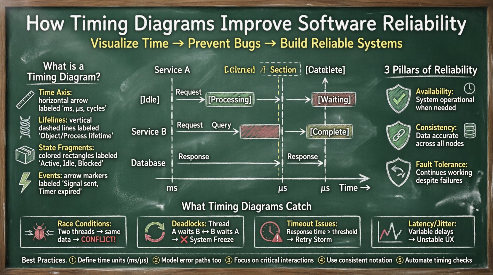
- Time Axis: Typically runs horizontally from left to right, representing the progression of time in milliseconds, microseconds, or clock cycles.
- Lifelines: Vertical bars representing the existence of an object or process over time.
- State Fragments: Rectangular areas on the lifeline indicating the state of the object (e.g., Active, Idle, Blocked, Processing).
- Events: Arrows or markers indicating when a specific action occurs, such as a signal being sent or a timer expiring.
By mapping these elements, developers create a timeline of system operations. This visual context is crucial for understanding how long a process takes to complete and how it waits for other processes. It transforms abstract logic into a tangible timeline that can be analyzed for errors.
🏗️ The Core Pillars of Software Reliability
Reliability in software engineering refers to the probability that a system will perform its required functions under stated conditions for a specified period. To achieve this, three main pillars must be addressed:
- Availability: The system must be operational when needed. Timing diagrams help verify that recovery processes complete within acceptable windows.
- Consistency: Data must remain accurate across distributed nodes. Visualizing write and read operations helps ensure data integrity is not compromised by latency.
- Fault Tolerance: The system must continue operating despite failures. Timing diagrams illustrate how long a fallback mechanism takes to engage, ensuring no service interruption is perceived by the user.
Without a clear understanding of time constraints, a system might be logically correct but practically unreliable. For instance, a database query might return the correct data, but if it takes 10 seconds to process, it violates the reliability requirement of a responsive user interface. Timing diagrams expose these temporal violations.
🐞 Detecting Race Conditions Through Visual Analysis
A race condition occurs when two or more processes access shared data concurrently, and the final outcome depends on the relative timing of their execution. These are notoriously difficult to debug because they are non-deterministic and often disappear when debuggers are attached.
Timing diagrams mitigate this risk by enforcing a strict visual order of events. When modeling a potential race condition, an engineer can draw the lifelines of the competing threads. If the diagram shows both threads attempting to write to the same memory location simultaneously without a synchronization barrier, the error is immediately visible.
- Visualizing Critical Sections: Highlight the duration where a resource is locked. If another process attempts access during this window, the diagram shows a conflict.
- Identifying Glitches: In hardware-software interfaces, signal glitches can occur if setup and hold times are not met. Timing diagrams explicitly show these windows.
- Ordering Dependencies: Ensure that initialization A completes before initialization B begins. The diagram forces a temporal check on this dependency.
By resolving these issues during the design phase, the likelihood of production failures drops significantly. It shifts the detection of concurrency bugs from runtime logs to design reviews.
🧵 Managing Concurrency and Thread Synchronization
Modern applications rely heavily on asynchronous processing to handle high loads. Threads, coroutines, and worker pools allow multiple tasks to run in parallel. However, synchronization primitives like mutexes, semaphores, and locks introduce their own timing complexities.
Timing diagrams assist in modeling these synchronization points. They help answer questions such as:
- How long does a thread wait for a lock before timing out?
- Does the lock acquisition time vary based on system load?
- Are there deadlocks where two threads wait for each other indefinitely?
When designing a multi-threaded application, engineers can sketch the state of each thread. If Thread A holds Resource 1 and waits for Resource 2, while Thread B holds Resource 2 and waits for Resource 1, a timing diagram can reveal the circular wait condition. This visual proof allows for the restructuring of resource acquisition logic before implementation begins.
Furthermore, timing diagrams clarify the behavior of priority inversion. In real-time systems, a high-priority task might be blocked by a low-priority task holding a lock. A timing diagram makes this priority inversion obvious, allowing architects to implement priority inheritance protocols.
🌐 Network Protocols and Handshake Verification
In distributed systems, network latency is a variable that cannot be ignored. Protocols like TCP/IP, HTTP/2, and gRPC rely on handshakes to establish connections. Timing diagrams are essential for validating these interactions.
Consider a standard three-way handshake (SYN, SYN-ACK, ACK). A timing diagram allows engineers to set a maximum allowable duration for this process. If the diagram shows the ACK taking longer than the configured timeout threshold, the connection is likely to fail under stress.
- Timeout Configuration: Define the exact millisecond duration for a request before a retry is triggered.
- Retransmission Logic: Visualize the gap between a failed packet and its retransmission to ensure it does not flood the network.
- Keep-Alive Intervals: Ensure the interval between keep-alive messages is shorter than the network idle timeout to prevent premature disconnection.
By modeling these network interactions, teams can ensure that their software handles network jitter gracefully. This prevents cascading failures where a slow response from one microservice causes the entire frontend to hang.
⚙️ Hardware-Software Interface Timing
Software reliability often hinges on how well it interacts with hardware. Embedded systems, IoT devices, and high-frequency trading platforms require precise timing. A delay of a few microseconds can result in data corruption or financial loss.
Interrupt Service Routines (ISRs) are a prime example. When a hardware interrupt occurs, the CPU must pause current tasks to handle it. A timing diagram maps out the interrupt latency (time from interrupt request to ISR entry) and the interrupt response time.
- Interrupt Latency: The time taken to acknowledge the interrupt.
- Context Switch Overhead: The time saved and restored during the ISR.
- Register Preservation: Ensuring that the state is saved before the ISR modifies it.
If the timing diagram shows that the ISR takes too long, it may block other critical interrupts. This visual analysis allows developers to optimize the ISR code or offload processing to a background thread, ensuring the real-time requirements are met.
📉 Identifying Latency and Jitter Issues
Latency is the delay before a transfer of data begins following an instruction for its transfer. Jitter is the variation in latency over time. Both are detrimental to user experience and system stability. Timing diagrams are the primary tool for analyzing these metrics.
When modeling a request-response cycle, engineers can mark the exact points where processing occurs. For example:
- Queue Wait Time: How long does a request sit in the buffer before processing?
- Processing Time: How long does the logic actually take to execute?
- Network Transit: How long does the data take to travel across the wire?
By summing these segments, the total latency is calculated. If the jitter is high, the timing diagram will show inconsistent spacing between events across multiple iterations. This inconsistency signals instability in the underlying infrastructure, prompting further investigation into resource contention or network congestion.
📝 Documenting System Interactions
Documentation is often overlooked in the pursuit of functionality, but it is vital for long-term reliability. Code changes frequently, and new team members join regularly. Timing diagrams serve as a durable reference for how the system behaves over time.
A well-maintained set of timing diagrams provides:
- Onboarding Material: New developers can understand the temporal flow without reading thousands of lines of code.
- Debugging Aid: When a bug occurs, engineers can compare the actual behavior against the documented timing diagram to spot deviations.
- Contract Definition: They define the expected behavior between services, acting as a contract for integration.
This documentation reduces the cognitive load on engineers during incident response. Instead of guessing the timing of events, they have a visual reference to follow.
⚠️ Common Timing Violations
Not all timing issues are created equal. Some are critical failures, while others are performance degradations. The table below categorizes common violations found in system modeling.
| Violation Type | Description | Impact on Reliability |
|---|---|---|
| Setup Time Violation | Data is not stable before the clock edge. | Unpredictable state changes, hardware failure. |
| Hold Time Violation | Data changes too soon after the clock edge. | Data corruption, metastability. |
| Timeout Expiry | Operation takes longer than the defined limit. | Service unavailability, retry storms. |
| Deadlock | Two processes wait on each other indefinitely. | System freeze, resource starvation. |
| Priority Inversion | High-priority task waits for low-priority task. | Missed deadlines, real-time failure. |
| Buffer Overflow | Data arrives faster than it can be consumed. | Packet loss, memory exhaustion. |
Reviewing these categories against your system’s timing diagrams helps prioritize which issues need immediate remediation. Hardware violations often require firmware updates, while software timeouts might require logic refactoring.
🔄 Integrating into the Development Lifecycle
To effectively use timing diagrams for reliability, they must be integrated into the software development lifecycle (SDLC). They should not be an afterthought added after deployment.
- Design Phase: Create high-level timing diagrams during system architecture reviews. Identify critical paths and timing constraints.
- Implementation Phase: Use timing diagrams to guide unit testing. Ensure that unit tests cover the timing boundaries, not just logical correctness.
- Integration Phase: Perform timing analysis on integrated components. Verify that the combined system meets the global timing requirements.
- Testing Phase: Use load testing tools to generate timing data. Compare the actual timing logs against the original diagrams.
- Maintenance Phase: Update diagrams when code changes affect timing. Ensure documentation remains synchronized with the codebase.
This integration ensures that timing considerations are part of the conversation at every stage, reducing the cost of fixing reliability issues later in the pipeline.
📊 Measuring Reliability Improvements
How do you quantify the benefit of using timing diagrams? While reliability is often measured in uptime percentages, timing diagrams contribute to specific metrics:
- Mean Time Between Failures (MTBF): By preventing race conditions and deadlocks, the frequency of failures decreases.
- Mean Time To Repair (MTTR): Better documentation and visual logs reduce the time needed to diagnose issues.
- Latency Percentiles: P99 and P999 latency become more stable when timing bottlenecks are identified early.
- Resource Utilization: Optimizing wait times reduces CPU idle time and improves overall throughput.
Tracking these metrics over time allows teams to see the direct correlation between rigorous timing modeling and system stability. It moves reliability from a qualitative goal to a quantitative reality.
💡 Summary of Best Practices
To maximize the impact of timing diagrams on software reliability, adhere to the following practices:
- Define Clear Time Units: Always specify the unit of time (ms, s, cycles) to avoid ambiguity.
- Include Error States: Model not just the happy path, but also timeout paths and error handling paths.
- Focus on Critical Paths: Do not diagram every single operation. Focus on the interactions that affect system stability.
- Use Consistent Notation: Adopt a standard notation for lifelines and events to ensure team-wide understanding.
- Automate Where Possible: Integrate timing analysis tools into the CI/CD pipeline to catch regressions automatically.
Software reliability is a continuous effort. It requires vigilance, precise modeling, and a deep understanding of how time affects system behavior. Timing diagrams provide the visual clarity needed to navigate this complexity. By adopting these practices, engineering teams can build systems that are not only functional but robust, predictable, and resilient against the unpredictable nature of time.
When you visualize time, you gain control over it. This control translates directly into reliability. As systems grow more distributed and complex, the ability to model temporal relationships becomes a competitive advantage. It separates systems that merely work from systems that work consistently under pressure.