Visualizing System Behavior: The Power of Timing Diagrams

In the complex architecture of digital systems, understanding the precise moment a signal changes state is critical. Timing diagrams provide a visual representation of how signals evolve over time. They are essential tools for engineers, developers, and designers who need to verify that components interact correctly. Without these visual aids, debugging asynchronous communication or verifying clock domains becomes a guessing game. This guide explores the mechanics, benefits, and applications of timing diagrams in system design.

What is a Timing Diagram? ⚙️

A timing diagram is a graph that displays the behavior of signals over a period. It maps the logical state of signals against a timeline. Unlike circuit schematics, which show physical connections, timing diagrams focus on the temporal relationship between events. They answer questions like: Does signal A change before signal B? Is the clock pulse wide enough? How long does data take to settle?

These diagrams are fundamental in:

• Verifying hardware protocols
• Documenting software logic interactions
• Debugging race conditions
• Validating clock and data alignment

Core Components of a Timing Diagram 🧩

To interpret a timing diagram effectively, one must understand its building blocks. Every diagram consists of specific elements that convey information about the system’s operation.

1. The Time Axis 📏

The horizontal axis represents time. It usually flows from left to right. The scale can be absolute (nanoseconds, microseconds) or relative (clock cycles). In synchronous systems, time is often divided into discrete steps corresponding to clock edges.

2. Signal Lines 📡

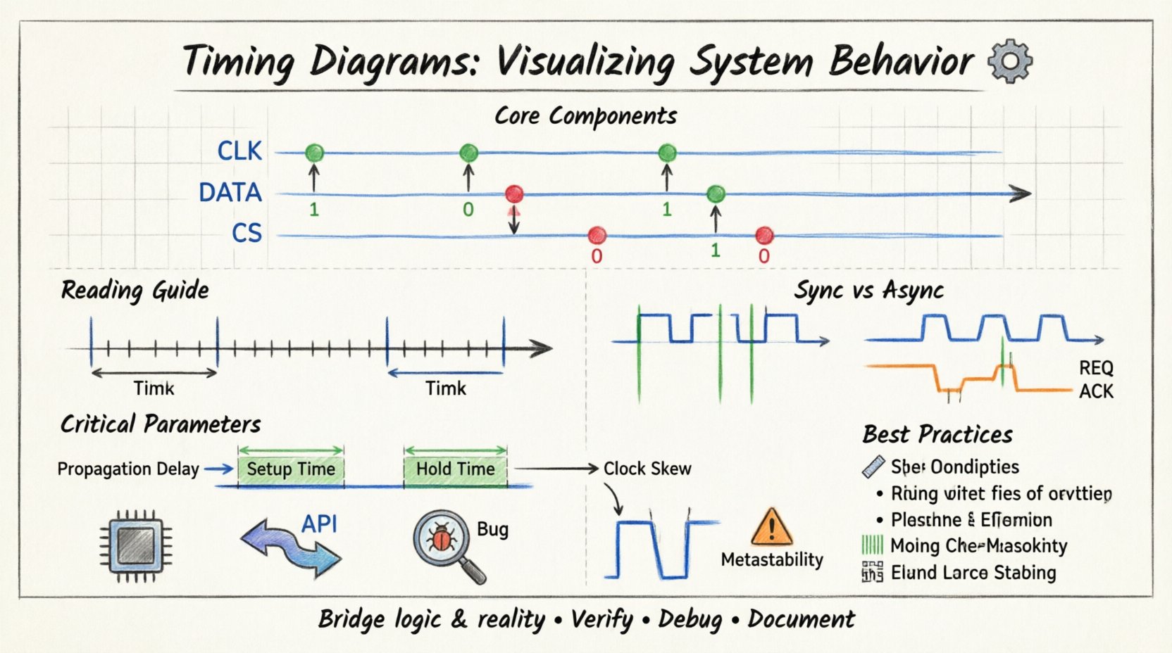
Each line represents a specific signal, wire, or data bus. These lines are labeled with names such as CLK, DATA, CS (Chip Select), or RST (Reset). The position of the line vertically separates different signals to avoid confusion.

3. Logic Levels 🟢🔴

Signals typically exist in discrete states. In digital logic, these are high (logic 1) and low (logic 0). Timing diagrams show transitions between these states. A transition from low to high is a rising edge. A transition from high to low is a falling edge.

4. Events and Transitions 🔄

Events are specific moments where a signal changes state. These are often marked by vertical lines or arrows. Important events include clock edges, data latches, and acknowledgment signals. The spacing between these events indicates duration.

Reading Timing Diagrams Effectively 👁️

Reading these diagrams requires a systematic approach. Misinterpreting the sequence of events can lead to design flaws. Follow these principles to ensure accuracy.

• Left to Right: Always read the timeline from the beginning (left) to the end (right). This represents the chronological flow of operations.
• Vertical Alignment: Events aligned vertically happen simultaneously. If two signals change at the exact same vertical line, they are concurrent.
• Duration: The horizontal length of a signal state indicates how long it stays in that state. A wide pulse means a longer duration.
• Dependencies: Look for cause and effect. One signal’s change often triggers another. The diagram shows the latency between these triggers.

Synchronous vs. Asynchronous Systems 🔄

Timing diagrams differ significantly depending on whether the system is synchronous or asynchronous. Understanding this distinction is vital for accurate analysis.

Synchronous Systems ⏰

These systems rely on a global clock signal. All state changes occur at specific clock edges (rising or falling). The diagram will show a regular clock pattern. Data is sampled only when the clock permits. This makes timing predictable but introduces constraints like setup and hold times.

Asynchronous Systems 🕰️

These systems do not rely on a global clock. State changes happen when input signals change. Timing diagrams here look less regular. They focus on handshaking protocols. One signal must go high, then the other, then back low. This requires careful analysis of delays to prevent race conditions.

Critical Parameters in Timing Analysis ⚙️

Beyond just drawing lines, engineers analyze specific parameters to ensure reliability. These parameters define the window in which a system functions correctly.

• Propagation Delay: The time it takes for a signal to travel from input to output through a component. This delay accumulates across logic gates.
• Setup Time: The minimum time before a clock edge that data must be stable. If data changes too late, the flip-flop cannot capture it correctly.
• Hold Time: The minimum time after a clock edge that data must remain stable. If data changes too soon, the current value is lost.
• Clock Skew: The difference in arrival time of the clock signal at different components. High skew can cause setup or hold violations.
• Metastability: A state where a flip-flop output is neither high nor low. This occurs when setup or hold times are violated. Timing diagrams help visualize the risk of metastability.

Application in Hardware and Software 🔌

Timing diagrams are not limited to hardware. They are used extensively in software architecture and protocol design as well.

Hardware Design

In hardware, these diagrams validate bus protocols. For example, verifying that the address bus is stable before the read strobe activates. They ensure that memory access times match the processor clock speed. They are also used to analyze power consumption spikes during signal transitions.

Software and Protocols

In software, timing diagrams map API calls or message exchanges. They show the sequence of requests and responses between services. This helps identify latency issues in distributed systems. They clarify the order of operations in multi-threaded environments.

Common Pitfalls and Errors 🛑

Creating or reading timing diagrams can lead to errors if not done carefully. Being aware of common mistakes helps improve accuracy.

• Ignoring Active Low: Many signals use active-low logic (inverted). A line dropping to low might mean the signal is active. Always check the legend or label.
• Assuming Instant Transitions: Real signals have rise and fall times. Ideal diagrams show vertical lines, but physical signals slope. This slope affects signal integrity.
• Overlooking Glitches: Short pulses that do not meet minimum width requirements can cause false triggers. These are often called glitches.
• Misinterpreting High-Z: High-impedance states mean a signal is disconnected. In diagrams, this looks like a dashed line or a specific symbol. Ignoring this can lead to bus contention errors.
• Incorrect Clock Alignment: Assuming all clocks are phase-aligned when they are not. Skew can cause data to be sampled incorrectly.

Comparison of Diagram Types 📊

Different contexts require different visualization methods. While timing diagrams are powerful, they are not the only tool.

Diagram Type	Primary Focus	Best Used For
Timing Diagram	Time and Signal States	Verifying clock/data relationships
State Diagram	System States	Defining logic flow and conditions
Sequence Diagram	Message Order	Software interactions and API calls
Circuit Schematic	Physical Connections	Wiring and component layout
Waveform Viewer	Real-Time Signals	Debugging actual hardware behavior

Best Practices for Documentation 📝

To make timing diagrams useful for teams and future reference, follow these best practices. Clear documentation reduces ambiguity and speeds up debugging.

• Label Everything: Every signal line must have a clear name. Avoid generic labels like Sig1.
• Include Units: Specify time units on the axis. Are we looking at milliseconds or clock cycles?
• Mark Critical Points: Highlight setup and hold windows explicitly. Use shading or distinct colors to mark critical timing windows.
• Keep it Organized: Group related signals together. For example, all control signals on top, data signals below.
• Document Assumptions: Note any assumptions made during creation. For example, assume zero propagation delay or specific load conditions.
• Use Consistent Notation: Stick to standard symbols for rising edges, falling edges, and high-impedance states.

Step-by-Step Guide to Creating a Diagram 🛠️

Creating a timing diagram from scratch requires a structured approach. Follow these steps to ensure completeness.

1. Identify Signals: List all inputs and outputs involved in the interaction.
2. Determine Sequence: Define the order of events. What triggers the process?
3. Set Time Scale: Decide on the granularity of the time axis.
4. Draw Clock: If synchronous, draw the clock signal first. It anchors the rest of the diagram.
5. Add Data: Plot the data signals relative to the clock edges.
6. Check Constraints: Verify setup and hold times against the drawn signals.
7. Review: Walk through the timeline to ensure no logical gaps exist.

The Role of Timing in Debugging 🐞

When a system fails, timing diagrams are often the first place engineers look. They help isolate whether the issue is logical or temporal. If the logic is correct but the timing is off, the system fails intermittently. This is often harder to reproduce than a hard logic error.

Debugging scenarios include:

• Data Corruption: Signals changing while being read.
• Missed Interrupts: An interrupt signal too short to be detected.
• Bus Contention: Two devices driving the bus at the same time.
• Clock Domain Crossing: Signals moving between different clock frequencies without proper synchronization.

Understanding Data Width and Alignment 📐

Timing diagrams also visualize data width. Parallel buses require multiple lines. Each line must transition in sync. Misalignment can cause data errors. The diagram shows how bits align within a clock cycle. For serial communication, the timing diagram shows the bit stream. It highlights the bit period and the sampling point.

Advanced Topics: Jitter and Noise 📉

Real-world signals are not perfect. Jitter is the deviation of the clock edge from its ideal position. Noise is random fluctuation in signal level. Timing diagrams can represent jitter by showing a thick band around the edge instead of a sharp line. This indicates uncertainty. Designers must ensure the system tolerates this uncertainty. The margin between the jitter band and the setup/hold window is the safety margin.

Integration with Test Suites 🧪

Timing diagrams are not just for design. They are used to generate test cases. Automated test suites can check if the actual system behavior matches the diagram. If the measured timing deviates beyond the tolerance, the test fails. This ensures that the hardware or software meets specifications throughout its lifecycle.

Conclusion on System Visualization 🎯

Timing diagrams remain a cornerstone of system engineering. They bridge the gap between abstract logic and physical reality. By visualizing the flow of time and signals, engineers can predict failures before they occur. They facilitate communication between hardware and software teams. A well-drawn diagram conveys more information than pages of text. As systems become faster and more complex, the need for precise timing analysis grows. Mastery of these diagrams ensures robust and reliable designs.

Remember to prioritize clarity and accuracy. Avoid assumptions. Verify every transition. With practice, reading and creating these diagrams becomes an intuitive part of the design process. They are the map that guides the traveler through the landscape of digital logic.