The Role of Timing Diagrams in System Design and Testing

Time is a fundamental dimension in every computing system. Whether you are building a high-frequency trading platform, a real-time embedded controller, or a distributed cloud service, the sequence and duration of events determine success or failure. While many focus on data flow and functionality, the temporal aspect often gets overlooked until performance issues arise. This guide explores the critical role of timing diagrams in system design and testing, providing a deep dive into how visualizing time improves architecture and reliability. 📊

Timing diagrams offer a specialized view of system behavior. They focus on the when rather than just the what. By mapping out state changes and signal transitions against a time axis, architects and testers can identify race conditions, bottlenecks, and latency violations before code is written or deployed. This approach shifts quality assurance left, catching temporal defects early in the development lifecycle. ⏱️

🔍 Understanding the Core Concept of Timing Diagrams

A timing diagram is a specific type of UML (Unified Modeling Language) interaction diagram. It emphasizes the time ordering of messages and state changes. Unlike sequence diagrams, which focus on the order of messages between objects, timing diagrams place a strong emphasis on the duration of events and the precise moment they occur. This distinction is vital for systems where milliseconds matter. 🛑

Key characteristics include:

• Time Axis: A horizontal axis represents the passage of time, flowing from left to right. This allows for the visualization of delays and concurrency.
• Lifelines: Vertical lines represent objects, components, or signals. These do not just show existence; they show the state of the entity over time.
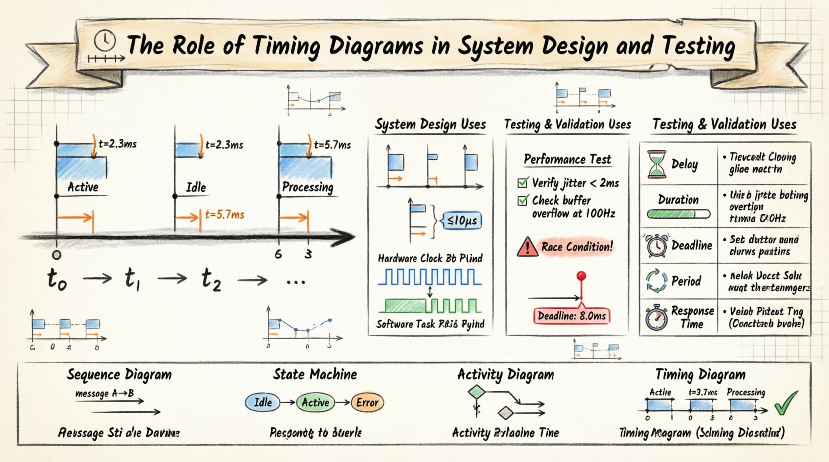
• State Changes: The diagram shows when an object enters a specific state, such as “Active,” “Idle,” or “Processing.”
• Signal Transitions: Arrows indicate the sending and receiving of signals, annotated with timestamps or durations.

When designing complex systems, understanding these elements prevents assumptions. For example, a developer might assume a response is instantaneous. A timing diagram forces the team to define exactly how long that response takes and what happens if it exceeds that limit. 🧠

⚙️ Timing Diagrams in System Design

During the design phase, timing diagrams serve as a blueprint for temporal constraints. They bridge the gap between abstract architecture and concrete implementation details. Here is how they influence design decisions.

1. Identifying Concurrency and Parallelism

Modern systems rarely run linearly. Multiple threads or processes often execute simultaneously. Timing diagrams make concurrency visible.

• Parallel Lifelines: When lifelines overlap horizontally, it indicates parallel execution. This helps designers spot potential race conditions where two processes access the same resource.
• Resource Contention: By visualizing when resources are locked or released, architects can optimize allocation strategies.
• Asynchronous Operations: These diagrams clarify how asynchronous callbacks interact with synchronous waiting periods.

2. Defining Latency Requirements

Latency is the time taken for a system to respond. Timing diagrams allow teams to set explicit boundaries.

• Maximum Delay: You can annotate a signal path with a maximum allowed duration. If the design implies a longer delay, the architecture must change.
• Minimum Delay: Some hardware protocols require a minimum wait time before a signal is sent. The diagram captures these physical constraints.
• Timeout Thresholds: Designers can define when a system should abort an operation if a response is not received within the specified time frame.

3. Hardware-Software Interface

In embedded systems, the interaction between code and hardware is strict. Timing diagrams are often the only way to document these interactions accurately.

• Clock Cycles: Designers can map signals to clock cycles, ensuring logic gates trigger at the right moment.
• Interrupt Handling: Diagrams show how interrupts pause normal processing and resume it later, accounting for the context switch time.
• Power States: Transitioning from sleep to active mode takes time. Timing diagrams plan for this latency to prevent data loss.

🧪 Timing Diagrams in Testing and Validation

Once the system is built, testing verifies that the temporal behavior matches the design. Timing diagrams become the reference standard for validation. 📏

1. Performance Testing

Load and stress testing often measure throughput, but timing diagrams measure precision. Testers can compare actual logs against the designed diagram.

• Latency Verification: Confirm that the time between a request and a response falls within the defined range.
• Throughput Analysis: While throughput is a rate, timing diagrams help visualize the gaps between transactions to ensure consistency.
• Jitter Measurement: Variability in timing is known as jitter. The diagram helps identify if jitter is within acceptable limits for the application.

2. Race Condition Detection

Race conditions occur when the outcome depends on the sequence of events. Timing diagrams expose these vulnerabilities.

• Overlapping Execution: If two critical operations overlap in a way that causes data corruption, the diagram highlights the risk.
• Order Violations: If a downstream process starts before an upstream process finishes, the diagram shows this violation clearly.
• Deadlock Scenarios: Cyclic dependencies with timing constraints can lead to deadlocks. Visualizing the wait times helps prevent this.

3. Real-Time System Validation

For real-time systems, missing a deadline is a failure. Timing diagrams are essential for compliance.

• Hard Deadlines: Events must occur by a specific time. The diagram defines the hard limit.
• Soft Deadlines: Events should occur by a time, but occasional misses are acceptable. The diagram helps quantify this tolerance.
• Periodicity: In periodic systems, the diagram ensures events repeat at regular intervals without drift.

📏 Key Components and Notation

To use timing diagrams effectively, one must understand the standard notation. Clarity in notation prevents misinterpretation during code reviews and testing. 📝

1. Lifelines

• Vertical lines representing the participant.
• Can represent a class instance, a thread, or a hardware pin.

2. State Bars

• Rectangular blocks on the lifeline indicating the current state of the object.
• Transitions occur when the state bar changes.

3. Messages

• Horizontal arrows indicating signals.
• Can be synchronous (blocking) or asynchronous (non-blocking).
• Often annotated with timestamps or durations.

4. Timing Constraints

• Annotations that define limits on time.
• Can specify exact values or ranges.

⏱️ Timing Constraints Explained

Timing constraints are the core value of these diagrams. They define the rules of engagement for time. Below is a table outlining common types of constraints used in system modeling. 📊

Constraint Type	Description	Example Scenario
Delay Constraint	Specifies the minimum or maximum time between two events.	A sensor must wait 10ms before sending data to avoid noise.
Duration Constraint	Defines how long a state must be maintained.	A button press must be held for 2 seconds to activate.
Deadline Constraint	Indicates the absolute time by which an event must complete.	A braking signal must reach the controller within 50ms.
Period Constraint	Defines the interval between repeated events.	Heartbeat signal sends every 1 second.
Response Time Constraint	Time elapsed between a trigger and a reaction.	System must respond to user login within 200ms.

Using these constraints explicitly removes ambiguity. It allows the testing team to write automated tests that assert these specific time boundaries. 🤖

🛑 Common Pitfalls and Solutions

Even with a powerful tool, mistakes happen. Recognizing common pitfalls ensures the diagrams remain useful assets rather than documentation clutter. 🧐

• Over-Complexity: Trying to model every millisecond can make the diagram unreadable. Focus on critical paths and timing-sensitive interactions.
• Lack of Context: A timing diagram without context is confusing. Always label the lifelines and define the time unit (e.g., ms, μs, clock cycles).
• Ignoring Network Variability: In distributed systems, network latency is not constant. Design diagrams should account for jitter and packet loss scenarios.
• Static vs. Dynamic: Timing diagrams are often static representations of dynamic behavior. Ensure the team understands that actual runtime behavior may vary due to garbage collection or OS scheduling.
• Outdated Diagrams: Code changes often invalidate diagrams. Treat them as living documents that require updates alongside the codebase.

🔄 Comparison with Other Modeling Techniques

Timing diagrams are not a replacement for other diagrams; they are a complement. Understanding when to use which tool is key to effective system modeling. 🧩

Diagram Type	Primary Focus	Best Used For
Sequence Diagram	Order of messages	High-level interaction flow, logical steps.
State Machine Diagram	State transitions	Logic flow, internal state management.
Activity Diagram	Workflow logic	Business processes, algorithm flow.
Timing Diagram	Time and duration	Real-time constraints, latency, concurrency.

For instance, a sequence diagram might show that “Service A calls Service B.” A timing diagram adds the detail: “Service A calls Service B, and Service B must reply within 100ms, or Service A times out.” Combining these views provides a complete picture of system behavior. 🌐

🚀 Strategic Implementation Steps

Integrating timing diagrams into your workflow requires a structured approach. Here is a recommended process to adopt this methodology effectively. 🛠️

1. Identify Critical Paths: Determine which interactions have strict time requirements. Not every API call needs a timing diagram.
2. Define Time Units: Agree on a standard unit of measurement across the team (milliseconds, microseconds, or clock cycles).
3. Collaborate on Constraints: Involve both architects and testers when defining timing constraints. Architects define the target; testers define the measurement capability.
4. Validate with Logs: Ensure that runtime logging captures enough detail to reconstruct the timing diagram for verification.
5. Iterate: As the system evolves, revisit the diagrams. Update them to reflect new latency characteristics or architectural changes.

This process ensures that timing diagrams remain relevant and actionable throughout the project lifecycle. It transforms them from static documentation into dynamic testing assets. 📈

🔗 Integrating with CI/CD Pipelines

Modern development relies on automation. Timing diagrams can be integrated into Continuous Integration and Continuous Deployment (CI/CD) pipelines to enforce quality gates. 🔄

• Automated Checks: Scripts can parse logs and verify that timing constraints defined in the diagrams are met during automated testing.
• Performance Gates: If a build exceeds the timing threshold defined in the diagram, the deployment can be blocked automatically.
• Regression Testing: Changes that inadvertently increase latency can be caught immediately if the timing diagram serves as the baseline for regression tests.

This integration shifts timing validation from a manual review activity to an automated enforcement mechanism. It ensures that performance is not an afterthought but a core requirement of every release. 🏁

The precision offered by timing diagrams is indispensable for systems where time is a critical resource. By explicitly modeling the temporal behavior, teams can build more robust, reliable, and predictable systems. Whether managing hardware interrupts or coordinating microservices, the discipline of timing analysis pays dividends in system stability. 🕒